0%

转载,整理自

1.MySQL 事务隔离级别和锁

2.对mysql乐观锁、悲观锁、共享锁、排它锁、行锁、表锁概念的理解

3.mysql乐观锁总结和实践:用version或者时间戳

事务及其特性

数据库事务(简称:事务)是数据库管理系统执行过程中的一个逻辑单位,由一个有限的数据库操作序列构成。事务的使用是数据库管理系统区别文件系统的重要特征之一。

事务拥有四个重要的特性:原子性(Atomicity)、一致性(Consistency)、隔离性(Isolation)、持久性(Durability),人们习惯称之为 ACID 特性。下面我逐一对其进行解释。

  • 原子性(Atomicity)

    事务开始后所有操作,要么全部做完,要么全部不做,不可能停滞在中间环节。事务执行过程中出错,会回滚到事务开始前的状态,所有的操作就像没有发生一样。例如,如果一个事务需要新增 100 条记录,但是在新增了 10 条记录之后就失败了,那么数据库将回滚对这 10 条新增的记录。也就是说事务是一个不可分割的整体,就像化学中学过的原子,是物质构成的基本单位。

  • 一致性(Consistency)

    指事务将数据库从一种状态转变为另一种一致的的状态。事务开始前和结束后,数据库的完整性约束没有被破坏。例如工号带有唯一属性,如果经过一个修改工号的事务后,工号变的非唯一了,则表明一致性遭到了破坏。

  • 隔离性(Isolation)

    要求每个读写事务的对象对其他事务的操作对象能互相分离,即该事务提交前对其他事务不可见。 也可以理解为多个事务并发访问时,事务之间是隔离的,一个事务不应该影响其它事务运行效果。这指的是在并发环境中,当不同的事务同时操纵相同的数据时,每个事务都有各自的完整数据空间。由并发事务所做的修改必须与任何其他并发事务所做的修改隔离。例如一个用户在更新自己的个人信息的同时,是不能看到系统管理员也在更新该用户的个人信息(此时更新事务还未提交)。

    注:MySQL 通过锁机制来保证事务的隔离性。

  • 持久性(Durability)

    事务一旦提交,则其结果就是永久性的。即使发生宕机的故障,数据库也能将数据恢复,也就是说事务完成后,事务对数据库的所有更新将被保存到数据库,不能回滚。这只是从事务本身的角度来保证,排除 RDBMS(关系型数据库管理系统,例如 Oracle、MySQL 等)本身发生的故障。

    注:MySQL 使用 redo log 来保证事务的持久性。

事务的隔离级别

SQL 标准定义的四种隔离级别被 ANSI(美国国家标准学会)和 ISO/IEC(国际标准)采用,每种级别对事务的处理能力会有不同程度的影响。

我们分别对四种隔离级别从并发程度由高到低进行描述,并用代码进行演示,数据库环境为 MySQL 5.7。

READ UNCOMMITTED(读未提交)

该隔离级别的事务会读到其它未提交事务的数据,此现象也称之为脏读

  1. 准备两个终端,在此命名为 mysql 终端 1 和 mysql 终端 2,再准备一张测试表test,写入一条测试数据并调整隔离级别为READ UNCOMMITTED,任意一个终端执行即可。

    1
    2
    3
    4
    5
    SET @@session.transaction_isolation = 'READ-UNCOMMITTED';
    create database test;
    use test;
    create table test(id int primary key);
    insert into test(id) values(1);
  1. 登录 mysql 终端 1,开启一个事务,将 ID 为1的记录更新为2。

    1
    2
    3
    begin;
    update test set id = 2 where id = 1;
    select * from test; -- 此时看到一条ID为2的记录
  2. 登录 mysql 终端 2,开启一个事务后查看表中的数据。

    1
    2
    3
    use test;
    begin;
    select * from test; -- 此时看到一条 ID 为 2 的记录

最后一步读取到了 mysql 终端 1 中未提交的事务(没有 commit 提交动作),即产生了脏读大部分业务场景都不允许脏读出现,是此隔离级别下数据库的并发是最好的

READ COMMITTED(读提交)

一个事务可以读取另一个已提交的事务,这次事务内多次读取会得到不一样的结果,此现象称为不可重复读(也称虚读)问题,Oracle 和 SQL Server 的默认隔离级别。

  1. 准备两个终端,在此命名为 mysql 终端 1 和 mysql 终端 2,再准备一张测试表test,写入一条测试数据并调整隔离级别为READ COMMITTED,任意一个终端执行即可。

    1
    2
    3
    4
    5
    SET @@session.transaction_isolation = 'READ-COMMITTED';
    create database test;
    use test;
    create table test(id int primary key);
    insert into test(id) values(1);
  2. 登录 mysql 终端 1,开启一个事务,将 ID 为1的记录更新为2,并确认记录数变更过来。

    1
    2
    3
    begin;
    update test set id = 2 where id = 1;
    select * from test; -- 此时看到一条记录为 2
  3. 登录 mysql 终端 2,开启一个事务后,查看表中的数据。

    1
    2
    3
    use test;
    begin;
    select * from test; -- 此时看一条 ID 为 1 的记录
  4. 登录 mysql 终端 1,提交事务。

    1
    commit;
  5. 切换到 mysql 终端 2。

    1
    select * from test; -- 此时看到一条 ID 为 2 的记录

mysql 终端 2 在开启了一个事务之后,在第一次读取 test 表(此时 mysql 终端 1 的事务还未提交)时 ID 为 1,在第二次读取 test 表(此时 mysql 终端 1 的事务已经提交)时 ID 已经变为 2,说明在此隔离级别下已经读取到已提交的事务。

REPEATABLE READ(可重复读)

该隔离级别是 MySQL 默认的隔离级别,在同一个事务里,select 的结果是事务开始时时间点的状态,因此,同样的 select 操作读到的结果会是一致的,但是,会有幻读现象。MySQL 的 InnoDB 引擎可以通过 next-key locks 机制(参考下文“行锁的算法”一节)来避免幻读。

  1. 准备两个终端,在此命名为 mysql 终端 1 和 mysql 终端 2,准备一张测试表test并调整隔离级别为REPEATABLE READ,任意一个终端执行即可。

    1
    2
    3
    4
    SET @@session.transaction_isolation = 'REPEATABLE-READ';
    create database test;
    use test;
    create table test(id int primary key,name varchar(20));
  2. 登录 mysql 终端 1,开启一个事务。

    1
    2
    begin;
    select * from test; -- 无记录
  3. 登录 mysql 终端 2,开启一个事务。

    1
    2
    begin;
    select * from test; -- 无记录
  4. 切换到 mysql 终端 1,增加一条记录并提交。

    1
    2
    insert into test(id,name) values(1,'a');
    commit;
  5. 切换到 msyql 终端 2。

    1
    select * from test; --此时查询还是无记录

    通过这一步可以证明,在该隔离级别下已经读取不到别的已提交的事务,如果想看到 mysql 终端 1 提交的事务,在 mysql 终端 2 将当前事务提交后再次查询就可以读取到 mysql 终端 1 提交的事务。我们接着实验,看看在该隔离级别下是否会存在别的问题。

  6. 此时接着在 mysql 终端 2 插入一条数据。

    1
    insert into test(id,name) values(1,'b'); -- 此时报主键冲突的错误

也许到这里您心里可能会有疑问,明明在第 5 步没有数据,为什么在这里会报错呢?其实这就是该隔离级别下可能产生的问题,MySQL 称之为幻读。注意我在这里强调的是 MySQL 数据库,Oracle 数据库对于幻读的定义可能有所不同。

SERIALIZABLE(序列化)

在该隔离级别下事务都是串行顺序执行的,MySQL 数据库的 InnoDB 引擎会给读操作隐式加一把读共享锁,从而避免了脏读、不可重读复读和幻读问题。

  1. 准备两个终端,在此命名为 mysql 终端 1 和 mysql 终端 2,分别登入 mysql,准备一张测试表 test 并调整隔离级别为SERIALIZABLE,任意一个终端执行即可。

    1
    2
    3
    4
    SET @@session.transaction_isolation = 'SERIALIZABLE';
    create database test;
    use test;
    create table test(id int primary key);
  2. 登录 mysql 终端 1,开启一个事务,并写入一条数据。

    1
    2
    begin;
    insert into test(id) values(1);
  3. 登录 mysql 终端 2,开启一个事务。

    1
    2
    begin;
    select * from test; -- 此时会一直卡住
  4. 立马切换到 mysql 终端 1,提交事务。

    1
    commit;

一旦事务提交,msyql 终端 2 会立马返回 ID 为 1 的记录,否则会一直卡住,直到超时,其中超时参数是由 innodb_lock_wait_timeout 控制。由于每条 select 语句都会加锁,所以该隔离级别的数据库并发能力最弱,但是有些资料表明该结论也不一定对,如果感兴趣,您可以自行做个压力测试。

表 1 总结了各个隔离级别下产生的一些问题。

表 1. 各个隔离级别下产生的一些问题
隔离级别 脏读(读到可能会回滚的数据) (一个事务内)不可重复读 幻读(读到数据不够新?)
读未提交 可以出现 可以出现 可以出现
读提交 不允许出现 可以出现 可以出现
可重复读 不允许出现 不允许出现 可以出现
序列化 不允许出现 不允许出现 不允许出现

脏读

脏读指在一个事务处理过程里读取了另一个未提交的事务中的数据,读取数据不一致。
事务A对数据进行增删改操作,但未提交,另一事务B可以读取到未提交的数据。如果事务A这时候回滚了,则第二个事务B读取的即为脏数据。

举例:当一个事务正在多次修改某个数据,而在这个事务中多次的修改都还未提交,这时一个并发的事务来访问该数据,就会造成两个事务得到的数据不一致。
例如:用户A向用户B转账100元,对应SQL命令如下:

1
2
update account set money = money + 100 where name=’B’;  --(此时A通知B)
update account set money = money - 100 where name=’A’;

当只执行第一条SQL时,A通知B查看账户,B发现确实钱已到账(此时即发生了脏读),而之后无论第二条SQL是否执行,只要该事务不提交,则所有操作都将回滚,那么当B以后再次查看账户时就会发现钱其实并没有转。

不可重复读(虚读)

所谓的虚读,也就是大家经常说的不可重复读,是指在数据库访问中,一个事务范围内两个相同的查询却返回了不同数据。这是由于查询时系统中其他事务修改的提交而引起的。比如事务T1读取某一数据,事务T2读取并修改了该数据,T1为了对读取值进行检验而再次读取该数据,便得到了不同的结果。
一种更易理解的说法是:在一个事务内,多次读同一个数据。在这个事务还没有结束时,另一个事务也访问该同一数据。那么,在第一个事务的两次读数据之间。由于第二个事务的修改,那么第一个事务读到的数据可能不一样,这样就发生了在一个事务内两次读到的数据是不一样的,因此称为不可重复读,即原始读取不可重复。

幻读

幻读是指当事务不是独立执行时发生的一种现象,例如第一个事务对一个表中的数据进行了修改,比如这种修改涉及到表中的“全部数据行”。同时,第二个事务也修改这个表中的数据,这种修改是向表中插入“一行新数据”。那么,以后就会发生操作第一个事务的用户发现表中还有没有修改的数据行,就好象发生了幻觉一样.

一般解决幻读的方法是增加范围锁RangeS,锁定检锁范围为只读,这样就避免了幻读。简单来说,幻读是由插入或者删除引起的。

不可重复读(虚读)和幻读比较

两者都表现为两次读取的结果不一致.

大致的区别在于不可重复读是由于另一个事务对数据的更改(update)所造成的,而幻读是由于另一个事务插入(insert)或删除(delete)引起的。

但如果你从控制的角度来看, 两者的区别就比较大:
对于前者, 只需要锁住满足条件的记录
对于后者, 要锁住满足条件及其相近的记录

MySQL 中的锁

锁也是数据库管理系统区别文件系统的重要特征之一。锁机制使得在对数据库进行并发访问时,可以保障数据的完整性和一致性。对于锁的实现,各个数据库厂商的实现方法都会有所不同。本文讨论 MySQL 中的 InnoDB 引擎的锁。

锁的类型

悲观锁(行锁)

InnoDB 实现了两种类型的行级锁,属于悲观锁的范畴:

  • 共享锁(也称为 S 锁,读锁):允许事务读取一行数据。

    可以使用 SQL 语句 select * from tableName where … lock in share mode; 手动加 S 锁。

  • 排他锁(也称为 X 锁,写锁,独占锁):允许事务删除或更新一行数据。

    可以使用 SQL 语句 select * from tableName where … for update; 手动加 X 锁。

S 锁和 S 锁是兼容的,X 锁和其它锁都不兼容.

举个例子,事务 T1 获取了一个行 r1 的 S 锁,另外事务 T2 可以立即获得行 r1 的 S 锁,此时 T1 和 T2 共同获得行 r1 的 S 锁,此种情况称为锁兼容,但是另外一个事务 T2 此时如果想获得行 r1 的 X 锁,则必须等待 T1 对行 r 锁的释放,此种情况也成为锁冲突

为了实现多粒度的锁机制,InnoDB 还有两种内部使用的意向锁,由 InnoDB 自动添加,且都是表级别的锁

  • 意向共享锁(IS):事务即将给表中的各个行设置共享锁S,事务给数据行加 S 锁前必须获得该表的 IS 锁。
  • 意向排他锁(IX):事务即将给表中的各个行设置排他锁X,事务给数据行加 X 锁前必须获得该表 IX 锁。

意向锁的主要目的是为了使得行锁表锁共存。表 2 列出了行级锁(S,X)和表级意向锁(IS,IX)的兼容性。

表 2. 行级锁和表级意向锁的兼容性
锁类型 X IX S IS
X 冲突 冲突 冲突 冲突
IX 冲突 兼容 冲突 兼容
S 冲突 冲突 兼容 兼容
IS 冲突 兼容 兼容 兼容

总结:意向锁(IX,IS)之间不会产生冲突, 其他情况可将IX锁当做X锁, IS锁当做S锁

乐观锁

乐观锁不是数据库自带的,需要我们自己去实现。乐观锁是指操作数据库时(更新操作),想法很乐观,认为这次的操作不会导致冲突,在操作数据时,并不加锁,而在进行更新后,再去判断是否有冲突了(CAS操作)。

一般来说有以下2种方式:

  1. 使用数据版本(Version)记录机制实现

    这是乐观锁最常用的一种实现方式。何谓数据版本?即为数据增加一个版本标识,一般是通过为数据库表增加一个数字类型的 “version” 字段来实现。当读取数据时,将version字段的值一同读出,数据每更新一次,对此version值加一。当我们提交更新的时候,判断数据库表对应记录的当前版本信息与第一次取出来的version值进行比对,如果数据库表当前版本号与第一次取出来的version值相等,则予以更新,否则认为是过期数据。

  2. 使用时间戳(Timestamp)记录机制实现

    乐观锁定的第二种实现方式和第一种差不多,同样是在需要乐观锁控制的table中增加一个字段,名称无所谓,字段类型使用时间戳(timestamp), 和上面的version类似,也是在更新提交的时候检查当前数据库中数据的时间戳和自己更新前取到的时间戳进行对比,如果一致则OK,否则就是版本冲突。

举例:在表中的数据进行操作时(更新),先给数据表加一个版本(version)字段,每操作一次,将那条记录的版本号加1。也就是先查询出那条记录,获取出version字段,如果要对那条记录进行操作(更新),则先判断此刻version的值是否与刚刚查询出来时的version的值相等,如果相等,则说明这段期间,没有其他程序对其进行操作,则可以执行更新,将version字段的值加1;如果更新时发现此刻的version值与刚刚获取出来的version的值不相等,则说明这段期间已经有其他程序对其进行操作了,则不进行更新操作。

下单操作包括3步骤:

1.查询出商品信息

1
select (status,status,version) from t_goods where id=#{id}

2.根据商品信息生成订单

3.修改商品status为2

1
2
3
update t_goods 
set status=2,version=version+1
where id=#{id} and version=#{version};

除了自己手动实现乐观锁之外,现在网上许多框架已经封装好了乐观锁的实现,如hiberate实现的乐观锁。

行锁的算法

InnoDB 存储引擎使用三种行锁的算法用来满足相关事务隔离级别的要求。

  • Record Locks

    该锁为索引记录上的锁,如果表中没有定义索引,InnoDB 会默认为该表创建一个隐藏的聚簇索引,并使用该索引锁定记录。

  • Gap Locks

    该锁会锁定一个范围,但是不括记录本身。可以通过修改隔离级别为 READ COMMITTED 或者配置 innodb_locks_unsafe_for_binlog 参数为 ON

  • Next-key Locks

    该锁就是 Record Locks 和 Gap Locks 的组合,即锁定一个范围并且锁定该记录本身。InnoDB 使用 Next-key Locks 解决幻读问题。需要注意的是,如果索引有唯一属性,则 InnnoDB 会自动将 Next-key Locks 降级为 Record Locks。举个例子,如果一个索引有 1, 3, 5 三个值,则该索引锁定的区间为 (-∞,1], (1,3], (3,5], (5,+ ∞)

死锁

死锁是指两个或两个以上的进程在执行过程中,由于竞争资源或者由于彼此通信而造成的一种阻塞的现象,若无外力作用,它们都将无法推进下去。此时称系统处于死锁状态或系统产生了死锁,这些永远在互相等待的进程称为死锁进程。

InnoDB 引擎采取的是 wait-for graph 等待图的方法来自动检测死锁,如果发现死锁会自动回滚一个事务。

下面我们通过一个示例来了解死锁。

  1. 准备两个终端,在此命名为 mysql 终端 1 和 mysql 终端 2,分别登入 mysql,再准备一张测试表test写入两条测试数据,并调整隔离级别为SERIALIZABLE,任意一个终端执行即可。

    1
    2
    3
    4
    5
    SET @@session.transaction_isolation = 'REPEATABLE-READ';
    create database test;
    use test;
    create table test(id int primary key);
    insert into test(id) values(1),(2);
  1. 登录 mysql 终端 1,开启一个事务,手动给 ID 为1的记录加 X 锁。

    1
    2
    begin;
    select * from test where id = 1 for update;
  2. 登录 mysql 终端 2,开启一个事务,手动给 ID 为2的记录加 X 锁。

    1
    2
    begin;
    select * from test where id = 2 for update;
  3. 切换到 mysql 终端 1,手动给 ID 为2的记录加 X 锁,此时会一直卡住,因为此时在等待第 3 步中 X 锁的释放,直到超时,超时时间由innodb_lock_wait_timeout控制。

    1
    select * from test where id = 2 for update;
  4. 在锁超时前立刻切换到 mysql 终端 2,手动给 ID 为1的记录加 X 锁,此时又会等待第 2 步中 X 所的释放,两个终端都在等待资源的释放,所以 InnoDB 引擎会立马检测到死锁产生,自动回滚一个事务,以防止死锁一直占用资源。

    1
    2
    select * from test where id = 1 for update;
    ERROR 1213 (40001): Deadlock found when trying to get lock; try restarting transaction

此时,通过 show engine innodb status\G 命令可以看到 LATEST DETECTED DEADLOCK 相关信息,即表明有死锁发生;或者通过配置 innodb_print_all_deadlocks(MySQL 5.6.2 版本开始提供)参数为 ON 将死锁相关信息打印到 MySQL 的错误日志。

锁的优化建议

锁如果利用不好,会给业务造成大量的卡顿现象,在了解了锁相关的一些知识点后,我们可以有意识的去避免锁带来的一些问题。

  1. 合理设计索引,让 InnoDB 在索引键上面加锁的时候尽可能准确,尽可能的缩小锁定范围,避免造成不必要的锁定而影响其他 Query 的执行。
  2. 尽可能减少基于范围的数据检索过滤条件,避免因为间隙锁带来的负面影响而锁定了不该锁定的记录。
  3. 尽量控制事务的大小,减少锁定的资源量和锁定时间长度。
  4. 在业务环境允许的情况下,尽量使用较低级别的事务隔离,以减少 MySQL 因为实现事务隔离级别所带来的附加成本。

结束语

通过阅读本文,可以让您对数据库的事务还有事务的隔离级别有个基本的了解,同时也介绍了 MySQL 中 InnoDB 引擎中一些锁相关的知识,从而可以让您利用关系型数据库系统设计一个更为健壮的业务模型。

参考资源

转载自详解布隆过滤器的原理,使用场景和注意事项

在进入正文之前,之前看到的有句话我觉得说得很好:

Data structures are nothing different. They are like the bookshelves of your application where you can organize your data. Different data structures will give you different facility and benefits. To properly use the power and accessibility of the data structures you need to know the trade-offs of using one.

大意是不同的数据结构有不同的适用场景和优缺点,你需要仔细权衡自己的需求之后妥善适用它们,布隆过滤器就是践行这句话的代表。

什么是布隆过滤器

本质上布隆过滤器是一种数据结构,比较巧妙的概率型数据结构(probabilistic data structure),特点是高效地插入和查询,可以用来告诉你 “某样东西一定不存在或者可能存在”

相比于传统的 List、Set、Map 等数据结构,它更高效、占用空间更少,但是缺点是其返回的结果是概率性的,而不是确切的。

实现原理

HashMap 的问题

讲述布隆过滤器的原理之前,我们先思考一下,通常你判断某个元素是否存在用的是什么?应该蛮多人回答 HashMap 吧,确实可以将值映射到 HashMap 的 Key,然后可以在 O(1) 的时间复杂度内返回结果,效率奇高。但是 HashMap 的实现也有缺点,例如存储容量占比高,考虑到负载因子的存在,通常空间是不能被用满的,而一旦你的值很多例如上亿的时候,那 HashMap 占据的内存大小就变得很可观了。

还比如说你的数据集存储在远程服务器上,本地服务接受输入,而数据集非常大不可能一次性读进内存构建 HashMap 的时候,也会存在问题。

布隆过滤器数据结构

布隆过滤器是一个 bit 向量或者说 bit 数组,长这样:

img

如果我们要映射一个值到布隆过滤器中,我们需要使用多个不同的哈希函数生成多个哈希值,并对每个生成的哈希值指向的 bit 位置 1,例如针对值 “baidu” 和三个不同的哈希函数分别生成了哈希值 1、4、7,则上图转变为:

img

Ok,我们现在再存一个值 “tencent”,如果哈希函数返回 3、4、8 的话,图继续变为:

img

值得注意的是,4 这个 bit 位由于两个值的哈希函数都返回了这个 bit 位,因此它被覆盖了。现在我们如果想查询 “dianping” 这个值是否存在,哈希函数返回了 1、5、8三个值,结果我们发现 5 这个 bit 位上的值为 0,说明没有任何一个值映射到这个 bit 位上,因此我们可以很确定地说 “dianping” 这个值不存在。而当我们需要查询 “baidu” 这个值是否存在的话,那么哈希函数必然会返回 1、4、7,然后我们检查发现这三个 bit 位上的值均为 1,那么我们可以说 “baidu” 存在了么?答案是不可以,只能是 “baidu” 这个值可能存在。

这是为什么呢?答案跟简单,因为随着增加的值越来越多,被置为 1 的 bit 位也会越来越多,这样某个值 “taobao” 即使没有被存储过,但是万一哈希函数返回的三个 bit 位都被其他值置位了 1 ,那么程序还是会判断 “taobao” 这个值存在。

支持删除么

感谢评论区提醒,传统的布隆过滤器并不支持删除操作。但是名为 Counting Bloom filter 的变种可以用来测试元素计数个数是否绝对小于某个阈值,它支持元素删除。可以参考文章 Counting Bloom Filter 的原理和实现

如何选择哈希函数个数和布隆过滤器长度

很显然,过小的布隆过滤器很快所有的 bit 位均为 1,那么查询任何值都会返回“可能存在”,起不到过滤的目的了。布隆过滤器的长度会直接影响误报率,布隆过滤器越长其误报率越小。

另外,哈希函数的个数也需要权衡,个数越多则布隆过滤器 bit 位置位 1 的速度越快,且布隆过滤器的效率越低;但是如果太少的话,那我们的误报率会变高。

img
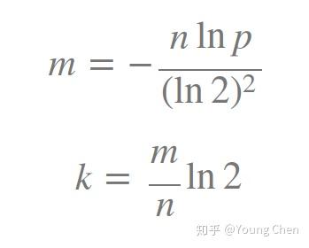
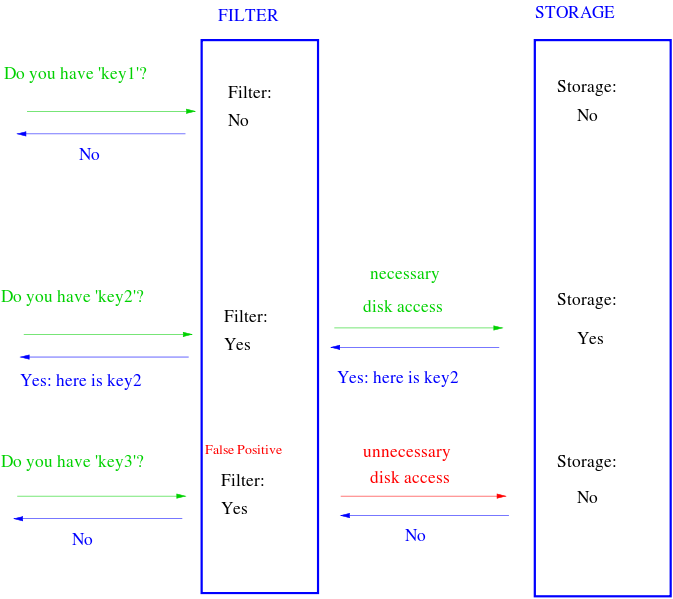
k 为哈希函数个数,m 为布隆过滤器长度,n 为插入的元素个数,p 为误报率

如何选择适合业务的 k 和 m 值呢,这里直接贴一个公式:

img

如何推导这个公式这里只是提一句,因为对于使用来说并没有太大的意义,你让一个高中生来推会推得很快。k 次哈希函数某一 bit 位未被置为 1 的概率为:

[公式]

插入n个元素后依旧为 0 的概率和为 1 的概率分别是:

[公式] [公式]

标明某个元素是否在集合中所需的 k 个位置都按照如上的方法设置为 1,但是该方法可能会使算法错误的认为某一原本不在集合中的元素却被检测为在该集合中(False Positives),该概率由以下公式确定

[公式]

最佳实践

常见的适用常见有,利用布隆过滤器减少磁盘 IO 或者网络请求,因为一旦一个值必定不存在的话,我们可以不用进行后续昂贵的查询请求。

另外,既然你使用布隆过滤器来加速查找和判断是否存在,那么性能很低的哈希函数不是个好选择,推荐 MurmurHash、Fnv 这些。

大Value拆分

Redis 因其支持 setbit 和 getbit 操作,且纯内存性能高等特点,因此天然就可以作为布隆过滤器来使用。但是布隆过滤器的不当使用极易产生大 Value,增加 Redis 阻塞风险,因此生成环境中建议对体积庞大的布隆过滤器进行拆分。

拆分的形式方法多种多样,但是本质是不要将 Hash(Key) 之后的请求分散在多个节点的多个小 bitmap 上,而是应该拆分成多个小 bitmap 之后,对一个 Key 的所有哈希函数都落在这一个小 bitmap 上。

参考资料

https://hackernoon.com/probabilistic-data-structures-bloom-filter-5374112a7832hackernoon.comBloom Filterswww.jasondavies.com图标

转载自Probabilistic Data structures: Bloom filter

If you have a glass-protected bookshelf, that will protect your books from dust and insects, but it will cost you more time to access the books when you need them. Because you first need to slide or open the glass and then can get the books. On the other hand, if it’s an open bookshelf, that will give you quicker access but you will lose the protection. Similarly, if you organize your books in lexicographic order of their name, you can easily search for a book if you know it’s name. But if your bookshelf has cases of different size and you organize your books based on their size, it will look nice, but can you find a book in a hurry? I don’t think so.

Data structures are nothing different. They are like the bookshelves of your application where you can organize your data. Different data structures will give you different facility and benefits. To properly use the power and accessibility of the data structures you need to know the trade-offs of using one.

When main-stream data structures like Lists, Maps, Sets, Trees etc. are mostly used for achieving certain results about whether the data exist or not, maybe along with their number of occurrences and such, Probabilistic data structures will give you memory-efficient, faster result with a cost of providing a ‘probable’ result instead of a ‘certain’ one. It might not seems intuitive to use such data structures for now, but I’ll try to convince you in this post that these type of data structures have their specific use cases and you might find them useful in certain scenarios.

In this post, I’ll talk about one of the most popular probabilistic data structures called ‘Bloom filter’. In future, I’ll try to write about some others.

Bloom filter

Do you know how hash tables work? When you insert a new data in a simple array or list, the index, where this data would be inserted, is not determined from the value to be inserted. That means there is no direct relationship between the ‘key(index)’ and the ‘value(data)’. As a result, if you need to search for a value in the array you have to search in all of the indexes. Now, in hash tables, you determine the ‘key’ or ‘index’ by hashing the ‘value’. Then you put this value in that index in the list. That means the ‘key’ is determined from the ‘value’ and every time you need to check if the value exists in the list you just hash the value and search on that key. It’s pretty fast and will require O(1) searching time in Big-O notation.

img

Now, let’s consider that you have a huge list of weak passwords and it is stored on some remote server. It’s not possible to load them at once in the memory/RAM because of the size. Each time a user enters his/her password you want to check if it is one of the weak passwords and if it is, you want to give him/her a warning to change it to something stronger. What can you do? As you already have the list of the weak passwords, you can store them in a hash table or something like that and each time you want to match, you can check against it if the given password has any match. The matching might be fast but the cost of searching it on the disk or over the network on a remote server would make it slow. Don’t forget that you would need to do it for every password given by every user. How can we reduce the cost?

Well, Bloom filter can help us here. How? I’m going to answer it after explaining how a bloom filter works. OK?

By definition, Bloom filter can check for if a value is ‘possibly in the set’ or ‘definitely not in the set’. The subtle difference between ‘possibly’ and ‘definitely not’ — is very crucial here. This ‘possibly in the set’ is exactly why it is called probabilistic. Using smart words it means that false positive is possible (there can be cases where it falsely thinks that the element is positive) but false negative is impossible. Don’t be impatient, we are explaining what does it actually mean, shortly.

The bloom filter essentially consists of a bit-vector or bit-list(a list containing only either 0 or 1-bit value) of length m, initially all values set to 0, as shown below.

img

Image Credit: GeeksforGeeks

To add an item to the bloom filter, we feed it to k different hash functions and set the bits to ‘1’ at the resulting positions. As you can see, in hash tables we would’ve used a single hash function and as a result get only a single index as output. But in the case of the bloom filter, we would use multiple hash functions, which would give us multiple indexes.

img

Image Credit: GeeksforGeeks

As you can see in the above example, for the given input ‘geeks’ our 3 hash functions will give 3 different output — 1, 4 and 7. We’ve marked them.

img

Image Credit: GeeksforGeeks

For another input ‘nerd’, the hash functions give us 3, 4 and 5. You might’ve noticed that the index ‘4’ is already marked by the previous ‘geeks’ input. Hold your thought, this point is interesting and we’re going to discuss it shortly.

We’ve already populated our bit vector with two inputs, now we can check for a value for its existence. How can we do that?
Easy. Just as we would’ve done it in a hash table. We would hash the ‘searched input’ with our 3 hash functions and see what are the resulting indexes hold.

img

Image Credit: GeeksforGeeks

So, searching for ‘cat’, our hash functions are giving us 1, 3 and 7 this time. And we can see that all of the indexes are already marked as 1. That means we can say, “maybe ‘cat’ is already inserted on our list”. But it didn’t. So, what’s went wrong?
Actually, nothing went wrong. The thing is, this is the case of a ‘false positive’. Bloom filter is telling us that it seems that maybe ‘cat’ was inserted before, because the indexes should’ve been marked by ‘cat’ are already marked (though by other different data).
So, if that’s the case, how it is helpful? Well, let’s consider if ‘cat’ would’ve given us the output of 1, 6, 7 instead of 1, 3, 7, what would happen then? We can see that among 3 indexes, 6 is ‘0’, that means it wasn’t marked by any of the previous inputs. That means obviously ‘cat’ never inserted before, if it was, there was no chance of 6 to be ‘0’, right? That’s how bloom filter can tell ‘certainly’ if a data is not on the list.

So, in a nutshell:

  • If we search for a value and see any of the hashed indexes for this value is ‘0’ then, the value is definitely not on the list.
  • If all of the hashed indexes is ‘1’ then ‘maybe’ the searched value is on the list.

Does it start making sense? A little maybe?

Fine, now, back to the ‘password’ example we were talking earlier. If we implement our weak password checking with this type of bloom filter, you can see that initially, we would mark our bloom filter with our list of passwords, which will give us a bit vector with some indexes marked as ‘1’ and others left as 0. As the size of the bloom filter won’t be very large and will be a fixed size, it can easily be stored in the memory and also on the client side if necessary. That’s why bloom filter is very space-efficient. Where a hash table requires being of arbitrary size based on the input data, the bloom filters can work well with a fixed size.
So, every time a user enters their password, we will feed it to our hash functions and check it against our bit vector. If the password is strong enough, the bloom filter will show us that the password is certainly not in the ‘weak password list’ and we don’t have to do any more query. But if the password seems weak and gives us a ‘positive’ (might be false positive) result we will then send it to our server and check our actual list to confirm.

As you can see, most of the time we don’t even need to make a request to our server or read from disk to check the list, this will be a significant improvement in speed of the application. In case, if we don’t want to store the bit-vector at the client side, we can still load it in the server memory and that will at least saves some disk lookup time. Also consider that, if your bloom filters false positive rate is 1%(we will talk about the error rate in details later), that means among the costly round-trips to the server or the disk, only 1% of the query will be returned with false result, other 99% won’t go in vain.
Not bad, huh?

img

Nice visual simulation about how bloom filters work. Image Credit: WikiPedia

Bloom filter operations

The basic bloom filter supports two operations: test and add.

Test is used to check whether a given element is in the set or not.

Add simply adds an element to the set.

Now a little quiz for you.

Based on what we’ve discussed so far, is it possible to Remove an item from the bloom filter? If yes, then how?

Take a 2 minutes break and think about the solution.

Got anything? Nothing? Let me help you a bit. Let’s bring back the bit-vector after inserting ‘geeks’ and ‘nerd’ in it.

img

Image Credit: GeeksforGeeks

img

Image Credit: GeeksforGeeks

Now we want to remove ‘geeks’ from it. So, if we remove 1, 4, 7 from the bit vector, as they are marked by ‘geeks’, and convert them to ‘0’, what will happen? You can easily see that, next time if we search for ‘nerd’, as the index ‘4’ will show ‘0’, it will definitely tell us that ‘nerd’ is not on the list, though it actually is. That means removal is impossible without introducing false negatives.

So, what’s the solution?

The solution is we can’t support Remove operation in this simple bloom filters. But if we really need to have a Removal functionality we can use a variation of the bloom filter known as ‘Counting bloom filter’. The idea is simple. Instead of storing a single bit of values, we will store an integer value and our bit vector will then be an integer vector. This will increase the size and costs more space to gives us the Removal functionality. Instead of just marking a bit value to ‘1’ when inserting a value, we will increment the integer value by 1. To check if an element exists, check if the corresponding indexes after hashing the element is greater than 0.
If you are having a hard time to understand how a ‘Counting bloom filter’ can give us ‘deletion’ feature, I’ll suggest you take a pen and a paper and simulate our bloom filter as a counting filter and then try a deletion on it. Hopefully, you’ll get it easily. If you failed, try again. If you failed again then please leave a comment and I’ll try to describe it.

Bloom filter size and number of Hash functions

You might already understand that if the size of the bloom filter is too small, soon enough all of the bit fields will turn into ‘1’ and then our bloom filter will return ‘false positive’ for every input. So, the size of the bloom filter is a very important decision to be made. A larger filter will have less false positives, and a smaller one more. So, we can tune our bloom filter to how much precise we need it to be based on the ‘false positive error rate’.
Another important parameter is ‘how many hash functions we will use’. The more hash functions we use, the slower the bloom filter will be, and the quicker it fills up. If we have too few, however, we may suffer too many false positives.

img

Image Credit: Abishek Bhat’s article about bloom filter

You can see from the above graph that, increasing the number of hash functions, k, will drastically reduce the error rate, p.

We can calculate the false positive error rate, p\, based on the size of the filter, m\, the number of hash functions, k\, and the number of elements inserted, n\, with the formula:

img

Seems like WTF? Don’t worry, we would actually mostly need to decide what our m\ and k\ would be. So, if we set an error tolerance value p\ and the number of elements n\ by ourselves we can use the following formulas to calculate these parameters:

img

Another important point I also need to mention here. As the sole purpose of using bloom filter is to search faster, we can’t use slow hash functions, right? Cryptographic hash functions such as Sha-1, MD5 won’t be good choice for bloom filters as they are a bit slow. So, the better choices from the faster hash function implementations would be murmur, the fnv series of hashes, Jenkins hashes and HashMix.

Applications

Bloom filter is all about testing Membership in a set. The classic example of using bloom filters is to reduce expensive disk (or network) lookups for non-existent keys. As we can see that bloom filters can search for a key in O(k) constant time, where k is the number of hash functions, it will be very fast to test non-existence of a key.

If the element is not in the bloom filter, then we know for sure we don’t need to perform the expensive lookup. On the other hand, if it is in the bloom filter, we perform the lookup, and we can expect it to fail some proportion of the time (the false positive rate).

For some more concrete examples:

  • You’ve seen in our given example that we could’ve use it to warn the user for weak passwords.
  • You can use bloom filter to prevent your users from accessing malicious sites.
  • Instead of making a query to an SQL database to check if a user with a certain email exists, you could first use a bloom filter for an inexpensive lookup check. If the email doesn’t exist, great! If it does exist, you might have to make an extra query to the database. You can do the same to search for if a ‘Username is already taken’.
  • You can keep a bloom filter based on the IP address of the visitors to your website to check if a user to your website is a ‘returning user’ or a ‘new user’. Some false positive value for ‘returning user’ won’t hurt you, right?
  • You can also make a Spell-checker by using bloom filter to track the dictionary words.
  • Want to know how Medium used bloom filter to decide if a user already read post? Read this mind-blowing, freaking awesome article about it.

Do you still think that you won’t ever need bloom filter? Well, we don’t use all of the algorithms we’ve learned in our everyday life. But maybe someday it might save your arse. Who knows? Learning a new thing never hurts, right?

转载自How does the default hashCode() work?

参考译文

In which scratching the surface of hashCode() leads to a speleology trip through the JVM source reaching object layout, biased locking, and surprising performance implications of relying on the default hashCode().

Abundant thanks to Gil Tene and Duarte Nunes reviewing drafts of this article and their very valuable insights, suggestions and edits. Any remaining errors are my own.

A trivial mystery

Last week at work I submitted a trivial change to a class, an implementation of toString() so logs would be meaningful. To my surprise, the change caused a ~5% coverage drop in the class. I knew that all new code was covered by existing unit tests so, what could be wrong? Comparing coverage reports a sharper colleague noticed that the implementation of hashCode() was covered before the change but not after. Of course, that made sense: the default toString() calls hashCode():

1
2
3
public String toString() {
return getClass().getName() + "@" + Integer.toHexString(hashCode());
}

After overriding toString(), our custom hashCode() was no longer being called. We were missing a test.

Everyone knew the default toString() but..

What is the default implementation of hashCode()?

The value returned by the default implementation of hashCode() is called identity hash code so I will use this term from now on to distinguish it from the hash provided by overriden implementations of hashCode(). FYI: even if a class overrides hashCode(), you can always get the identity hash code of an object o by calling System.identityHashCode(o).

Common wisdom is that the identity hash code uses the integer representation of the memory address. That’s also what the J2SE JavaDocs for Object.hashCode() imply:

1
2
3
... is typically implemented by converting the internal address of
the object into an integer, but this implementation technique is not
required by the Java™ programming language.

Still, this seems problematic as the method contract requires that:

1
2
3
Whenever it is invoked on the same object more than once during an
execution of a Java application, the hashCode method must consistently
return the same integer.

Given that the JVM will relocate objects (e.g. during garbage collection cycles due to promotion or compaction), after we calculate an object’s identity hash we must be able to retain it in a way that survives object relocation.

A possibility could be to take the current memory position of the object on the first call to hashCode(), and save it somewhere along with the object, like the object’s header. That way, if the object is moved to a different memory location, it would carry the original hash with it. A caveat of this method is that it won’t prevent two objects from having the same identity hash, but that’s allowed by the spec.

The best confirmation would be to to look at the source. Unfortunately, the default java.lang.Object::hashCode() is a native function:

1
public native int hashCode();

Helmets on.

Will the real hashCode() please stand up

Note that the identity hashCode() implementation is dependant on the JVM. Since I will only look at OpenJDK sources, you should assume this specific implementation whenever I talk about the JVM. All links refer to changeset 5820:87ee5ee27509 of the Hotspot tree, I assume that most of it will also be applicable to Oracle’s JVM, but things could (in fact, are) different in others (more about this later.)

OpenJDK defines entry points for hashCode() at src/share/vm/prims/jvm.h and src/share/vm/prims/jvm.cpp. The latter has:

1
2
3
4
5
508 JVM_ENTRY(jint, JVM_IHashCode(JNIEnv* env, jobject handle))
509 JVMWrapper("JVM_IHashCode");
510 // as implemented in the classic virtual machine; return 0 if object is NULL
511 return handle == NULL ? 0 : ObjectSynchronizer::FastHashCode (THREAD, JNIHandles::resolve_non_null(handle)) ;
512 JVM_END

ObjectSynchronizer::FastHashCode() is also called from identity_hash_value_for, which is used from a few other call sites (e.g.: System.identityHashCode())

1
2
3
708 intptr_t ObjectSynchronizer::identity_hash_value_for(Handle obj) {
709 return FastHashCode (Thread::current(), obj()) ;
710 }

One might naively expect ObjectSynchronizer::FastHashCode() to do something like:

1
2
3
4
if (obj.hash() == 0) {
obj.set_hash(generate_new_hash());
}
return obj.hash();

But it turns out to be a hundred line function that seems to be far more complicated. At least we can spot a couple of if-not-exists-generate blocks like:

1
2
3
4
5
6
7
8
9
685   mark = monitor->header();
...
687 hash = mark->hash();
688 if (hash == 0) {
689 hash = get_next_hash(Self, obj);
...
701 }
...
703 return hash;

Which seems to confirm our hypothesis. Let’s ignore that monitor for now, and be satisfied that it gives us the object header. It is kept at mark, a pointer to an instance of markOop, which represents the mark word that belongs in the low bits of the object header. So, tries to get a hash inside the mark word. If it’s not there, it’s generated using get_next_hash, saved, and returned.

The actual identity hash generation

As we saw, this happens at get_next_hash. This function offers six methods based on the value of some hashCode variable.

1
2
3
4
5
6
0. A randomly generated number.
1. A function of memory address of the object.
2. A hardcoded 1 (used for sensitivity testing.)
3. A sequence.
4. The memory address of the object, cast to int.
5. Thread state combined with xorshift (https://en.wikipedia.org/wiki/Xorshift)

So what’s the default method? OpenJDK 8 seems to default on 5 according to globals.hpp:

1
2
1127   product(intx, hashCode, 5,                                                \
1128 "(Unstable) select hashCode generation algorithm") \

OpenJDK 9 keeps the same default. Looking at previous versions, both OpenJDK 7 and OpenJDK 6 use the first method, a random number generator.

So, unless I’m looking at the wrong place the default hashCode implementation in OpenJDK has nothing to do with the memory address, at least since version 6.

Object headers and synchronization

Let’s go back a couple of points that we left unexamined. First, ObjectSynchronizer::FastHashCode() seems overly complex, needing over 100 lines to perform what we though was a trivial get-or-generate operation. Second, who is this monitor and why does it have our object’s header?

The structure of the mark word is a good place to start making progress. In OpenJDK, it looks like this

1
2
3
4
5
6
7
8
9
10
11
12
13
14
15
16
17
18
19
20
21
22
23
24
25
30 // The markOop describes the header of an object.
31 //
32 // Note that the mark is not a real oop but just a word.
33 // It is placed in the oop hierarchy for historical reasons.
34 //
35 // Bit-format of an object header (most significant first, big endian layout below):
36 //
37 // 32 bits:
38 // --------
39 // hash:25 ------------>| age:4 biased_lock:1 lock:2 (normal object)
40 // JavaThread*:23 epoch:2 age:4 biased_lock:1 lock:2 (biased object)
41 // size:32 ------------------------------------------>| (CMS free block)
42 // PromotedObject*:29 ---------->| promo_bits:3 ----->| (CMS promoted object)
43 //
44 // 64 bits:
45 // --------
46 // unused:25 hash:31 -->| unused:1 age:4 biased_lock:1 lock:2 (normal object)
47 // JavaThread*:54 epoch:2 unused:1 age:4 biased_lock:1 lock:2 (biased object)
48 // PromotedObject*:61 --------------------->| promo_bits:3 ----->| (CMS promoted object)
49 // size:64 ----------------------------------------------------->| (CMS free block)
50 //
51 // unused:25 hash:31 -->| cms_free:1 age:4 biased_lock:1 lock:2 (COOPs && normal object)
52 // JavaThread*:54 epoch:2 cms_free:1 age:4 biased_lock:1 lock:2 (COOPs && biased object)
53 // narrowOop:32 unused:24 cms_free:1 unused:4 promo_bits:3 ----->| (COOPs && CMS promoted object)
54 // unused:21 size:35 -->| cms_free:1 unused:7 ------------------>| (COOPs && CMS free block)

The format is slightly different on 32 and 64 bits. The latter has two variants depending on whether Compressed Object Pointers are enabled. Both Oracle and OpenJDK 8 do by default.

Object headers may thus relate to a free block or an actual object, in which case there are multiple possible states. In the simplest, (“normal object”) the identity hash is stored directly in the low addresses of the header.

But in other states, we find a pointer to a JavaThread or a PromotedObject. The plot thickens: if we put the identity hash in a “normal object”, will someone take it away? Where? If the object is biased, where can we get/set the hash? What is a biased object?

Let’s try to answer those questions.

Biased locking

Biased objects appear as a result of Biased Locking. A (patented!) feature enabled by default from HotSpot 6 that tries to alleviate the cost of locking objects. Such operations are expensive because their implementation often relies on atomic CPU instructions (CAS) in order to safely handle lock/unlock requests on the object from different threads. It was observed that in most applications, the majority of objects are only ever locked by one thread so paying the cost of the atomic operation was often a waste. To avoid it, JVMs with biased locking allow threads to try and “bias” an object towards themselves. While an object is biased, the lucky thread can lock/unlock the object without atomic instructions. As long as there are no threads contending for the same object, we’ll gain performance.

The biased_lock bit in the header indicates whether an object is biased by the thread pointed at by JavaThread*. The lock bits indicate whether the object is locked.

Precisely because OpenJDK’s implementation of biased locking requires writing a pointer in the mark word, it also needs to relocate the real mark word (which contains the identity hash.)

This could explain the additional complexity in FastHashCode. The header not only holds the identity hash code, but also locking state (like the pointer to the lock’s owner thread). So we need to consider all cases and find where the identity hash resides.

Let’s go read FastHashCode. The first thing we find is:

1
2
3
4
5
6
7
8
9
601 intptr_t ObjectSynchronizer::FastHashCode (Thread * Self, oop obj) {
602 if (UseBiasedLocking) {
610 if (obj->mark()->has_bias_pattern()) {
...
617 BiasedLocking::revoke_and_rebias(hobj, false, JavaThread::current());
...
619 assert(!obj->mark()->has_bias_pattern(), "biases should be revoked by now");
620 }
621 }

Wait. It just revoked existing biases, and disabled biased locking on the object (the false means “don’t attempt rebias”). A few lines down, this is indeed an invariant:

1
2
637   // object should remain ineligible for biased locking
638 assert (!mark->has_bias_pattern(), "invariant") ;

If I’m reading correctly, this means that simply asking for the identity hash code of an object will disable biased locking, which in turn forces any attempt to lock the object to use expensive atomic instructions. Even if there is only one thread.

Oh boy.

Why does keeping biased locking state conflict with keeping the identity hash code?

To answer this question we must understand which are the possible locations of the mark word (that contains the identity hash) depending on the lock state of the object. The transitions are illustrated in this diagram from the HotSpot Wiki:

img

My (fallible) reasoning is the following.

For the 4 states at the top of the diagram, the OpenJDK will be able to use “thin” lock representations. In the simplest case (no locks) this means having the identity hash and other data directly in the object’s space for the mark word:

1
46 //  unused:25 hash:31 -->| unused:1   age:4    biased_lock:1 lock:2 (normal object)

in more complex cases, it needs that space to keep a pointer to the “lock record”. The mark word will thus be “displaced” and put somewhere else.

While we have only one thread trying to lock the object, that pointer will actually refer to a memory location in the thread’s own stack. Which is twice good: it’s fast (no contention or coordination to access that memory location), and it suffices for the thread to identify that it owns the lock (because the memory location points to its own stack.)

But this won’t work in all cases. If we have contended objects (e.g. objects used on synchronized statements that many threads traverse) we will need a more complex structure that fits not only a copy of the object’s header (again, “displaced”), but also a list of waiters. A similar need for a list of waiters appears if a thread executes object.wait().

This richer data structure is the ObjectMonitor, which is referred to as a the “heavyweight” monitor in the diagram. The value left in the object’s header doesn’t point to a “displaced mark word” anymore, but to an actual object (the monitor). Accessing the identity hash code will now require “inflating the monitor”: chasing a pointer to an object and reading/mutating whichever field contains the displaced mark word. Which is more expensive and requires coordination.

FastHashCode does have work to do.

Lines L640 to L680 deal with finding the header and checking for a cached identity hash. I believe these are a fast path that probe for cases that don’t need to inflate the monitor.

From L682 it needs to bite the bullet:

1
2
3
4
5
6
7
682   // Inflate the monitor to set hash code
683 monitor = ObjectSynchronizer::inflate(Self, obj);

684 // Load displaced header and check it has hash code
685 mark = monitor->header();
...
687 hash = mark->hash();

At this point, if the id. hash is there (hash != 0), the JVM can return. Otherwise we’ll get one from get_next_hash and safely store it in the displaced header kept by the ObjectMonitor.

This seems to offer a reasonable explanation to why calling hashCode() on an object of a class that doesn’t override the default implementation makes the object ineligible for biased locking:

  • In order to keep the identity hash of an object consistent after relocation we need to store the hash in the object’s header.
  • Threads asking for the identity hash may not even care about locking the object, but in practise they will be sharing data structures used by the locking mechanism. This is a complex beast in itself that might be not only mutating, but also moving (displacing) the header contents.
  • Biased locking helped perform lock/unlock operations without atomic operations, and this was effective as long as only one thread locked the object because we could keep the lock state in the mark word. I’m not 100% sure here, but I understand that since other threads may ask for the identity hash, even if there is a single thread interested in the lock, the header word will be contended and require atomic operations to be handled correctly. Which defeats the whole point of biased locking.

Recap

  • The default
1
hashCode()

implementation (identity hash code)

has nothing to do with the object’s memory address

, at least in OpenJDK. In versions 6 and 7 it is a randomly generated number. In 8 and, for now, 9, it is a number based on the thread state.

Here

is a test that yields the same conclusion.

  • Proving that “implementation-dependent” warns are not aesthetic: Azul’s Zing does generate the identity hash from the object’s memory address.
  • In HotSpot, the result of the identity hash generation is generated once, and cached in the

mark word

of the object’s header.

  • Zing uses a different solution to keep it consistent despite object relocations, in which they delay storing the id. hash until the object relocates. At that point, it’s stored in a “pre-header”
  • In HotSpot, calling the default
1
hashCode()

, or

1
System.identityHashCode()

will make the object ineligible for biased locking.

  • This implies that if you are synchronizing on objects that have no contention, you’d better override the default hashCode() implementation or you’ll miss out on JVM optimizations.
  • It is possible

to disable biased locking in HotSpot, on a per-object basis.

  • This can be very useful. I’ve seen applications very heavy on contended producer/consumer queues where biased locking was causing more trouble than benefit, so we disabled the feature completely. Turns out, we could’ve done this only on specific objects/classes simply by calling System.identityHashCode() on them.
  • I have found no HotSpot flag that allows changing the default generator, so experimenting with other options might need to compile from source

    .

Benchmarks

I wrote a simple JMH harness to verify those conclusions.

The benchmark (source) does something equivalent to this:

1
2
3
4
5
6
object.hashCode();
while(true) {
synchronized(object) {
counter++;
}
}

One configuration (withIdHash) synchronizes on an object that uses the identity hash, so we expect that biased locking will be disabled as soon as hashCode() is invoked. A second configuration (withoutIdHash) implements a custom hash code so biased locking should not be disabled. Each configuration is ran first with one thread, then with two threads (these have the suffix “Contended”.)

By the way, we must enable -XX:BiasedLockingStartupDelay=0 as otherwise the JVM will take 4s to trigger the optimisation distorting the results.

The first execution:

1
2
3
4
5
Benchmark                                       Mode  Cnt       Score      Error   Units
BiasedLockingBenchmark.withIdHash thrpt 100 35168,021 ± 230,252 ops/ms
BiasedLockingBenchmark.withoutIdHash thrpt 100 173742,468 ± 4364,491 ops/ms
BiasedLockingBenchmark.withIdHashContended thrpt 100 22478,109 ± 1650,649 ops/ms
BiasedLockingBenchmark.withoutIdHashContended thrpt 100 20061,973 ± 786,021 ops/ms

We can see that the using a custom hash code makes the lock/unlock loop work 4x faster than the one using the identity hash code (which disables biased locking.) When two threads contend for the lock, biased locking is disabled anyway so there is no significative difference between both hash methods.

A second run disables biased locking (-XX:-UseBiasedLocking) in all configurations.

1
2
3
4
5
Benchmark                                       Mode  Cnt      Score      Error   Units
BiasedLockingBenchmark.withIdHash thrpt 100 37374,774 ± 204,795 ops/ms
BiasedLockingBenchmark.withoutIdHash thrpt 100 36961,826 ± 214,083 ops/ms
BiasedLockingBenchmark.withIdHashContended thrpt 100 18349,906 ± 1246,372 ops/ms
BiasedLockingBenchmark.withoutIdHashContended thrpt 100 18262,290 ± 1371,588 ops/ms

The hash method no longer has any impact and withoutIdHash loses its advantage.

(All benchmarks were ran on a 2,7 GHz Intel Core i5.)

References

Whatever is not wild speculation and my weak reasoning trying to make sense of the JVM sources, comes from stitching together various sources about layout, biased locking, etc. The main ones are below:

转载自java默认的hashcode方法到底得到的是什么?

hashcode方法会影响jvm性能?听上去天方夜谭,实际上蕴藏着一些微小的原理,接下来让我们走进hashcode方法,一探native方法源头。

默认实现是什么?

调用hashCode方法默认返回的值被称为identity hash code(标识哈希码),接下来我们会用标识哈希码来区分重写hashCode方法。如果一个类重写了hashCode方法,那么通过调用System.identityHashCode(Object o)方法获得标识哈希码。

在hashCode方法注释中,说hashCode一般是通过对象内存地址映射过来的。

1
2
3
4
5
6
As much as is reasonably practical, the hashCode method defined by
class {@code Object} does return distinct integers for distinct
objects. (This is typically implemented by converting the internal
address of the object into an integer, but this implementation
technique is not required by the
Java<font size="-2"><sup>TM</sup></font> programming language.)

但是了解jvm的同学肯定知道,不管是标记复制算法还是标记整理算法,都会改变对象的内存地址。鉴于jvm重定位对象地址,但该hashCode又不能变化,那么该值一定是被保存在对象的某个地方了。

我们推测,很有可能是在第一次调用hashCode方法时获取当前内存地址,并将其保存在对象的某个地方,当下次调用时,只用从对象的某个地方获取值即可。但这样实际是有问题的,你想想,如果对象被归集到别的内存上了,那在对象以前的内存上创建的新对象其hashCode方法返回的值岂不是和旧对象的一样了?这倒没关系,java规范允许这样做。

以上都是我们的猜测,并没有实锤。我们来看一下源码吧,可恶,hashCode方法是一个本地方法。

1
public native int hashCode();

真正的hashCode方法

hashCode方法的实现依赖于jvm,不同的jvm有不同的实现,我们目前能看到jvm源码就是OpenJDK的源码,OpenJDK的源码大部分和Oracle的JVM源码一致。

OpenJDK定义hashCode的方法在src/share/vm/prims/jvm.hsrc/share/vm/prims/jvm.cpp

jvm.cpp:

1
2
3
4
5
508 JVM_ENTRY(jint, JVM_IHashCode(JNIEnv* env, jobject handle))
509 JVMWrapper("JVM_IHashCode");
510 // as implemented in the classic virtual machine; return 0 if object is NULL
511 return handle == NULL ? 0 : ObjectSynchronizer::FastHashCode (THREAD, JNIHandles::resolve_non_null(handle)) ;
512 JVM_END

ObjectSynchronizer :: FastHashCode() 也是通过调用identity_hash_value_for方法返回值的,System.identityHashCode()调用的也是这个方法。

1
2
3
708 intptr_t ObjectSynchronizer::identity_hash_value_for(Handle obj) {
709 return FastHashCode (Thread::current(), obj()) ;
710 }

我们可能会认为 ObjectSynchronizer :: FastHashCode() 会判断当前的hash值是否为0,如果是0则生成一个新的hash值。实际上没那么简单,来看看其中的代码。

1
2
3
4
5
6
7
8
9
685   mark = monitor->header();
...
687 hash = mark->hash();
688 if (hash == 0) {
689 hash = get_next_hash(Self, obj);
...
701 }
...
703 return hash;

上边的片段展示了hash值是如何生成的,可以看到hash值是存放在对象头中的,如果hash值不存在,则使用get_next_hash方法生成。

真正的 identity hash code 生成

在第二节中,我们终于找到了生成hash的最终函数 get_next_hash,这个函数提供了6种生成hash值的方法。

1
2
3
4
5
6
0. A randomly generated number.
1. A function of memory address of the object.
2. A hardcoded 1 (used for sensitivity testing.)
3. A sequence.
4. The memory address of the object, cast to int.
5. Thread state combined with xorshift (https://en.wikipedia.org/wiki/Xorshift)

那么默认用哪一个呢?根据globals.hpp,OpenJDK8默认采用第五种方法。而 OpenJDK7OpenJDK6 都是使用第一种方法,即 随机数生成器

大家也看到了,JDK的注释算是欺骗了我们,明明在678版本上都是随机生成的值,为什么要引导说是内存地址映射呢?我理解可能以前就是通过第4种方法实现的。

对象头格式

在上一节,我们知道了hash值是放在对象头里的,那就来了解一下对象头的结构吧。

markOop.hpp

1
2
3
4
5
6
7
8
9
10
11
12
13
14
15
16
17
18
19
20
21
22
23
24
25
30 // The markOop describes the header of an object.
31 //
32 // Note that the mark is not a real oop but just a word.
33 // It is placed in the oop hierarchy for historical reasons.
34 //
35 // Bit-format of an object header (most significant first, big endian layout below):
36 //
37 // 32 bits:
38 // --------
39 // hash:25 ------------>| age:4 biased_lock:1 lock:2 (normal object)
40 // JavaThread*:23 epoch:2 age:4 biased_lock:1 lock:2 (biased object)
41 // size:32 ------------------------------------------>| (CMS free block)
42 // PromotedObject*:29 ---------->| promo_bits:3 ----->| (CMS promoted object)
43 //
44 // 64 bits:
45 // --------
46 // unused:25 hash:31 -->| unused:1 age:4 biased_lock:1 lock:2 (normal object)
47 // JavaThread*:54 epoch:2 unused:1 age:4 biased_lock:1 lock:2 (biased object)
48 // PromotedObject*:61 --------------------->| promo_bits:3 ----->| (CMS promoted object)
49 // size:64 ----------------------------------------------------->| (CMS free block)
50 //
51 // unused:25 hash:31 -->| cms_free:1 age:4 biased_lock:1 lock:2 (COOPs && normal object)
52 // JavaThread*:54 epoch:2 cms_free:1 age:4 biased_lock:1 lock:2 (COOPs && biased object)
53 // narrowOop:32 unused:24 cms_free:1 unused:4 promo_bits:3 ----->| (COOPs && CMS promoted object)
54 // unused:21 size:35 -->| cms_free:1 unused:7 ------------------>| (COOPs && CMS free block)

它的格式在32位和64位上略有不同,64位有两种变体,具体取决于是否启用了压缩对象指针。

对象头中偏向锁和hashcode的冲突

在上一节我们看到,normal object和biased object分别存放的是hashcode和java的线程id。因此也就是说如果调用了本地方法hashCode,就会占用偏向锁对象使用的位置,偏向锁将会失效,晋升为轻量级锁。

这个过程我们可以看看这个图

upload successful

这里我来简单解读一下,首先在jvm启动时,可以使用-XX:+UseBiasedLocking=true参数开启偏向锁。

接下来,如果偏向锁可用,那分配的对象中标记字格式为可包含线程ID,当未锁定时,线程ID为0,第一次获取锁时,线程会把自己的线程ID写到ThreadID字段内,这样,下一次获取锁时直接检查标记字中的线程ID和自身ID是否一致,如果一致就认为获取了锁,因此不需要再次获取锁。

假设这时有别的线程需要竞争锁了,此时该线程会通知持有偏向锁的线程释放锁,假设持有偏向锁的线程已经销毁,则将对象头设置为无锁状态,如果线程活着,则尝试切换,如果不成功,那么锁就会升级为轻量级锁。

这时有个问题来了,如果需要获取对象的identity hash code,偏向锁就会被禁用,然后给原先设置线程ID的位置写入hash值。

如果hash有值,或者偏向锁无法撤销,则会进入轻量级锁。轻量级锁竞争时,每个线程会先将hashCode值保存到自己的栈内存中,然后通过CAS尝试将自己新建的记录空间地址写入到对象头中,谁先写成功谁就拥有了该对象。

轻量级锁竞争失败的线程会自旋尝试获取锁一段时间,一段时间过后还没获取到锁,则升级为重量级锁,没获取锁的线程会被真正阻塞。

总结

  • OpenJDK默认的hashCode方法实现和对象内存地址无关,在版本6和7中,它是随机生成的数字,在版本8中,它是基于线程状态的数字。(AZUL-ZING的hashcode是基于地址的)
  • 在Hotspot中,hash值会存在标记字中。
  • hashCode方法和System.identityHashCode()会让对象不能使用偏向锁,所以如果想使用偏向锁,那就最好重写hashCode方法。
  • 如果大量对象跨线程使用,可以禁用偏向锁。
  • 使用-XX:hashCode=4来修改默认的hash方法实现。

参考

历史

linux下的进程通信手段基本上是从Unix平台上的进程通信手段继承而来的。而对Unix发展做出重大贡献的两大主力AT&T的贝尔实验室及BSD(加州大学伯克利分校的伯克利软件发布中心)在进程间通信方面的侧重点有所不同。前者对Unix早期的进程间通信手段进行了系统的改进和扩充,形成了“system V IPC”,通信进程局限在单个计算机内;后者则跳过了该限制,形成了基于套接口(socket)的进程间通信机制。Linux则把两者继承了下来,如图示:

img

其中,最初Unix IPC包括:管道、FIFO、信号;System V IPC包括:System V消息队列、System V信号灯、System V共享内存区;Posix IPC包括: Posix消息队列、Posix信号灯、Posix共享内存区。

有两点需要简单说明一下:

  • 由于Unix版本的多样性,电子电气工程协会(IEEE)开发了一个独立的Unix标准,这个新的ANSI Unix标准被称为计算机环境的可移植性操作系统界面(POSIX)。现有大部分Unix和流行版本都是遵循POSIX标准的,而Linux从一开始就遵循POSIX标准;

  • BSD并不是没有涉足单机内的进程间通信(socket本身就可以用于单机内的进程间通信)。

事实上,很多Unix版本的单机IPC留有BSD的痕迹,如4.4BSD支持的匿名内存映射、4.3+BSD对可靠信号语义的实现等等。

图一给出了linux 所支持的各种IPC手段,在本文接下来的讨论中,为了避免概念上的混淆,在尽可能少提及Unix的各个版本的情况下,所有问题的讨论最终都会归结到Linux环境下的进程间通信上来。并且,对于Linux所支持通信手段的不同实现版本(如对于共享内存来说,有Posix共享内存区以及System V共享内存区两个实现版本),将主要介绍Posix API。

简介

linux下进程间通信的几种主要手段简介:

管道(Pipe)及有名管道(named pipe)

管道可用于具有亲缘关系进程间的通信,有名管道克服了管道没有名字的限制,因此,除具有管道所具有的功能外,它还允许无亲缘关系进程间的通信;

信号(Signal)

信号是比较复杂的通信方式,用于通知接受进程有某种事件发生,除了用于进程间通信外,进程还可以发送信号给进程本身;linux除了支持Unix早期信号语义函数sigal外,还支持语义符合Posix.1标准的信号函数sigaction(实际上,该函数是基于BSD的,BSD为了实现可靠信号机制,又能够统一对外接口,用sigaction函数重新实现了signal函数);

报文(Message)队列(消息队列)

消息队列是消息的链接表,包括Posix消息队列system V消息队列。有足够权限的进程可以向队列中添加消息,被赋予读权限的进程则可以读走队列中的消息。消息队列克服了信号承载信息量少,管道只能承载无格式字节流以及缓冲区大小受限等缺点。

共享内存

使得多个进程可以访问同一块内存空间,是最快的可用IPC形式。是针对其他通信机制运行效率较低而设计的。往往与其它通信机制,如信号量结合使用,来达到进程间的同步及互斥。

信号量(semaphore)

主要作为进程间以及同一进程不同线程之间的同步手段。

套接口(Socket)

更为一般的进程间通信机制,可用于不同机器之间的进程间通信。起初是由Unix系统的BSD分支开发出来的,但现在一般可以移植到其它类Unix系统上:Linux和System V的变种都支持套接字。

一般来说,linux下的进程包含以下几个关键要素:有一段可执行程序;有专用的系统堆栈空间;内核中有它的控制块(进程控制块),描述进程所占用的资源,这样,进程才能接受内核的调度;具有独立的存储空间进程和线程有时候并不完全区分,而往往根据上下文理解其含义。

补充

  • 管道:管道中还有命名管道和非命名管道之分,非命名管道只能用于父子进程通讯,命名管道可用于非父子进程,命名管道就是FIFO,管道是先进先出的通讯方式。FIFO是一种先进先出的队列。它类似于一个管道,只允许数据的单向流动。每个FIFO都有一个名字,允许不相关的进程访问同一个FIFO,因此也成为命名管。
  • 消息队列:是用于两个进程之间的通讯,首先在一个进程中创建一个消息队列,然后再往消息队列中写数据,而另一个进程则从那个消息队列中取数据。需要注意的是,消息队列是用创建文件的方式建立的,如果一个进程向某个消息队列中写入了数据之后,另一个进程并没有取出数据,即使向消息队列中写数据的进程已经结束,保存在消息队列中的数据并没有消失,也就是说下次再从这个消息队列读数据的时候,就是上次的数据!
  • 信号量, 不能传递复杂消息,只能用来同步
  • 共享内存,只要首先创建一个共享内存区,其它进程按照一定的步骤就能访问到这个共享内存区中的数据,当然可读可写;

​ 几种方式的比较:

  • ​ 管道:速度慢,容量有限
  • ​ 消息队列:容量受到系统限制,且要注意第一次读的时候,要考虑上一次没有读完数据的问题。
  • ​ 信号量:不能传递复杂消息,只能用来同步
  • ​ 共享内存区:能够很容易控制容量,速度快,但要保持同步,比如一个进程在写的时候,另一个进程要注意读写的问题,相当于线程中的线程安全,当然,共享内存区同样可以用作线程间通讯,不过没这个必要,线程间本来就已经共享了一块内存的。

本文整理自

深刻理解Linux进程间通信(IPC)

进程间通信

仅做个人学习总结所用,遵循CC 4.0 BY-SA版权协议,如有侵权请联系删除!

死锁概念和产生原因

死锁是指多个进程循环等待彼此占有的资源而无限期的僵持等待下去的局面。原因是:

  • 系统提供的资源太少了,远不能满足并发进程对资源的需求
  • 进程推进顺序不合适,互相占有彼此需要的资源,同时请求对方占有的资源,往往是程序设计不合理

死锁产生的必要条件

需要同时具有以下四个条件:

  • 互斥条件:即某个资源在一段时间内只能由一个进程占有,不能同时被两个或两个以上的进程占有
  • 不可抢占条件:进程所获得的资源在未使用完毕之前,资源申请者不能强行的从资源占有者手中夺取资源,而只能由该资源的占有者进程自行释放
  • 占有且等待条件:进程至少已经占有了一个资源,但又申请了一个新的被其他进程所占有的资源,此时处于等待状态
  • 循环等待条件:若干个进程形成环形链,每个都占用对方申请的下一个资源

只要系统发生死锁,这些条件必然成立,而只要上述条件之一不满足,就不会发生死锁。

死锁的处理策略

为使系统不发生死锁,必须设法破坏产生死锁的四个必要条件之一,或者允许死锁产生,但当死锁发生时能检测出思索,并有能力实现恢复。
一般有死锁的预防、死锁避免、死锁的检测与恢复三种方法。
(1) 死锁预防:破坏导致死锁必要条件中的任意一个就可以预防死锁。例如,要求用户申请资源时一次性申请所需要的全部资源,这就破坏了保持和等待条件;将资源分层,得到上一层资源后,才能够申请下一层资源,它破坏了环路等待条件。预防通常会降低系统的效率

(2) 死锁避免:避免是指进程在每次申请资源时判断这些操作是否安全,例如,使用银行家算法。死锁避免算法的执行会增加系统的开销。允许前三个必要条件,但通过明智的选择,确保永远不会到达死锁点,因此死锁避免比死锁预防允许更多的并发。

(3) 死锁检测:不须实现采取任何限制性措施,而是允许系统在运行过程发生死锁,但可通过系统设置的检测机构及时检测出死锁的发生,并精确地确定于死锁相关的进程和资源,然后采取适当的措施,从系统中将已发生的死锁清除掉。死锁预防和避免都是事前措施,而死锁的检测则是判断系统是否处于死锁状态,如果是,则执行死锁解除策略。

(4) 死锁解除:这是与死锁检测结合使用的,它使用的方式就是剥夺。即将某进程所拥有的资源强行收回,分配给其他的进程。常用方法:撤销或挂起一些进程,以便回收一些资源,再将这些资源分配给已处于阻塞状态的进程。死锁检测盒解除有可能使系统获得较好的资源利用率和吞吐量,但在实现上难度也最大。

死锁预防:

  • 打破互斥条件:允许进程同时访问资源(有些资源就是不可以同时访问的,它是设备的固有属性所决定的,不仅不能改变,还应该加以保证。无实用价值)
  • 打破不可抢占条件:比如给进程设置优先级,高优先级的可以抢占资源(实现困难,降低系统性能)
  • 打破占有且等待条件:实行资源预分配策略,即进程在运行前一次性的向系统申请它所需要的全部资源(不可预测资源的使用,利用率低,降低并发性)
  • 破坏循环等待条件:把资源事先分类编号,按优先级分配,使进程在申请,占用资源时不会形成环路。所有进程对资源的请求必须严格按资源序号递增的顺序提出(限制和编号实现困难,增加系统开销,有些资源暂时不用也需要先申请,增加了进程对资源的占用时间)

死锁避免

允许进程动态的申请资源,但系统在进行资源分配前,应先计算此次资源分配的安全性。若此次分配不会导致系统进入不安全状态,则将资源你分配给进程,否则,让进程等待。
所谓安全状态,是指系统能按某种进程推进顺序,为每个进程分配其所需的资源,直至满足每个进程对资源的最大需求,是每个进程都可以顺序的完成。此时成P1P2P3…为安全序列,如果系统无法找到一个安全序列,则称系统处于不安全状态。
并非所有的不安全状态都是死锁状态,但当系统进入不安全状态后,便可能进入死锁状态;反之,只要系统处于安全状态,系统便可以避免进入死锁状态。

银行家算法是最著名的死锁避免算法。

(1)两种死锁避免算法:

进程启动拒绝:如果一个进程的请求会导致死锁,则不启动该进程。

资源分配拒绝:如果一个进程增加的资源请求会导致死锁,则不允许此分配(银行家算法)。

(2)银行家算法

1.如果request<=need,转向步骤2;否则认为出错,因为请求资源大于需要资源。

2.如果request<=available,转向步骤3,;否则尚无足够资源,进程p阻塞;

3.系统尝试为把资源分配给进程P,并修改available、allocation和need的数值。

4.系统执行安全性算法,检查此次分配后系统是否处于安全状态,若安全,才正式将资源分配给进程P,否则将本次试探性分配作废,让进程P等待。

死锁的检测

资源分配图&&死锁定理

死锁解除

1)资源剥夺法。挂起某些思索进程,并抢占它的资源,将这些资源分配给其他的死锁进程。但应防止被挂起的进程长时间得不到资源时,而处于资源匮乏的状态。
2)进程撤销法。强制撤销一个或一部分进程并剥夺这些进程的资源。撤销的原则可以按进程的优先级和撤销进程代价的高低进行。
3)进程回退法。让一个或多个进程回退到足以回避死锁的地步,进程回退时资源释放资源而不是被剥夺。要求系统保持进程的历史信息,设置还原点。

题目描述

在数组中的两个数字,如果前面一个数字大于后面的数字,则这两个数字组成一个逆序对。输入一个数组,求出这个数组中的逆序对的总数P。并将P对1000000007取模的结果输出。 即输出P%1000000007

输入描述:

1
题目保证输入的数组中没有的相同的数字数据范围:	对于%50的数据,size<=10^4	对于%75的数据,size<=10^5	对于%100的数据,size<=2*10^5

示例1

输入

1
1,2,3,4,5,6,7,0

输出

1
7

解答

归并排序.leetcode上可以通过,牛客网剑指Offer没有完全通过,由于错误用例看不完整,正在排查原因

1
2
3
4
5
6
7
8
9
10
11
12
13
14
15
16
17
18
19
20
21
22
23
24
25
26
27
28
29
30
31
32
33
34
35
36
37
38
39
40
41
42
43
44
45
46
47
48
49
int c = 0;

public int InversePairs(int[] array) {
if (array == null || array.length <= 1) {
return 0;
}
mergeSort(array);
return c % 1000000007;
}

private int[] mergeSort(int[] n) {
if (n.length <= 1) {
return n;
} else if (n.length == 2) {
if (n[0] > n[1]) {
c++;
int t = n[0];
n[0] = n[1];
n[1] = t;
}
return n;
}

int[] n1, n2;
n1 = mergeSort(Arrays.copyOfRange(n, 0, n.length / 2));
n2 = mergeSort(Arrays.copyOfRange(n, n.length / 2, n.length));

//todo merge 统计逆序对
int[] n3 = new int[n.length];
int i = 0, j = 0, k = 0;
while (i < n1.length && j < n2.length) {
if (n1[i] <= n2[j]) {
n3[k] = n1[i];
i++;
} else {
n3[k] = n2[j];
j++;
c += (n1.length - i);
}
k++;
}
for (; i < n1.length; k++, i++) {
n3[k] = n1[i];
}
for (; j < n2.length; k++, j++) {
n3[k] = n2[j];
}
return n3;
}

官方题解

链接:https://www.nowcoder.com/questionTerminal/96bd6684e04a44eb80e6a68efc0ec6c5?answerType=1&f=discussion
来源:牛客网

题目描述:给定一个数组arr, 数组元素各不相同,求arr[i] > arr[j] 且 i < j的个数。

首先还是提出两个问题,带着问题来看题解,我觉得效率更好。
Q1:为什么归并排序需要额外的空间?
Q2:为什么此题的最优解法可以借助归并排序的思想?

方法一:暴力方法

对于此题,按住一个arr[i], 依次判断{i+1 … n-1]是否满足条件。n为数组的大小。
代码如下:

1
2
3
4
5
6
7
8
9
10
11
12
13
14
15
16
17
18
19
class Solution {
private:
const int kmod = 1000000007;
public:
int InversePairs(vector<int> data) {
int ret = 0;
int n = data.size();
for (int i = 0; i < n; ++i) {
for (int j = i + 1; j < n; ++j) {
if (data[i] > data[j]) {
ret += 1;
ret %= kmod;
}
}
}

return ret;
}
};

对于10^5数据,O(N^2)算法显然超时。
时间复杂度:O(N^2)
空间复杂度:O(1)

方法二:归并排序思想

A1: 首先回答一下第一个问题,为什么归并排序需要额外空间?
显然我们知道,归并排序的过程就是,递归划分整个区间为基本相等的左右区间,之间左右区间各只有一个数字,然后就合并两个有序区间。
问题就出在了合并两个有序区间上,需要额外的空间。
为什么呢?
这里我举个例子,比如需要合并的两个有序区间为[3 4] 和 [1 2]
我们需要得到最后的结果为[1 2 3 4], 如果不需要额外的空间的话,是做不到的,
当比较1 和 3 的时候, 1 比 3 小,就会覆盖原来的位置。

A2:回答第二个问题之前,先了解一下归并排序的过程,主要有以下两个操作:

  • 递归划分整个区间为基本相等的左右两个区间
  • 合并两个有序区间

可能看了代码,更好理解:

1
2
3
4
5
6
7
8
9
10
11
12
13
14
15
16
17
18
19
20
21
22
23
24
25
26
27
28
29
30
31
32
33
34
35
36
37
38
39
40
41
42
43
44
// 合并过程
void merge__(vector<int> &arr, int l, int mid, int r) {
// 在这个地方创建额外空间,是一种不好的做法,更好的做法,等下讲
vector<int> tmp(r - l + 1);
int i = l, j = mid + 1, k = 0;

while (i <= mid && j <= r) {
if (arr[i] >= arr[j]) {
tmp[k++] = arr[j++];
}
else {
tmp[k++] = arr[i++];
}
}

while (i <= mid) {
tmp[k++] = arr[i++];
}
while (j <= r) {
tmp[k++] = arr[j++];
}

for (k = 0, i = l; i <= r; ++i, ++k) {
arr[i] = tmp[k];
}
}

// 递归划分过程
void merge_sort__(vector<int> &arr, int l, int r) {
// 只有一个数字,则停止划分
if (l >= r) {
return;
}

int mid = l + ((r - l) >> 1);
merge_sort__(arr, l, mid);
merge_sort__(arr, mid + 1, r);
// 合并两个有序区间
merge__(arr, l, mid, r);
}
// 要排序的数组 arr
void merge_sort(vector<int>& arr) {
merge_sort__(arr, 0, arr.size() - 1);
}

明白了归并排序的过程,那么回答问题2.
如果两个区间为[4, 3] 和[1, 2]
那么逆序数为(4,1),(4,2),(3,1),(3,2),同样的如果区间变为有序,比如[3,4] 和 [1,2]的结果是一样的,也就是说区间有序和无序结果是一样的。
但是如果区间有序会有什么好处吗?当然,如果区间有序,比如[3,4] 和 [1,2]
如果3 > 1, 显然3后面的所有数都是大于1, 这里为 4 > 1, 明白其中的奥秘了吧。所以我们可以在合并的时候利用这个规则。

直接上代码:

1
2
3
4
5
6
7
8
9
10
11
12
13
14
15
16
17
18
19
20
21
22
23
24
25
26
27
28
29
30
31
32
33
34
35
36
37
38
39
40
41
42
43
44
45
46
47
48
49
50
class Solution {
private:
const int kmod = 1000000007;
public:
int InversePairs(vector<int> data) {
int ret = 0;
merge_sort__(data, 0, data.size() - 1, ret);
return ret;
}


void merge_sort__(vector<int> &arr, int l, int r, int &ret) {
if (l >= r) {
return;
}

int mid = l + ((r - l) >> 1);
merge_sort__(arr, l, mid, ret);
merge_sort__(arr, mid + 1, r, ret);
merge__(arr, l, mid, r, ret);
}

void merge__(vector<int> &arr, int l, int mid, int r, int &ret) {
vector<int> tmp(r - l + 1);
int i = l, j = mid + 1, k = 0;

while (i <= mid && j <= r) {
if (arr[i] > arr[j]) {
tmp[k++] = arr[j++];
// 奥妙之处
ret += (mid - i + 1);
ret %= kmod;
}
else {
tmp[k++] = arr[i++];
}
}

while (i <= mid) {
tmp[k++] = arr[i++];
}
while (j <= r) {
tmp[k++] = arr[j++];
}

for (k = 0, i = l; i <= r; ++i, ++k) {
arr[i] = tmp[k];
}
}
};

刚才提到在函数内部开辟额外空间的做法很不好。因为这样会涉及到频繁的构建 vector 和析构vector,所以比较好的做法是:直接在最外层开辟一个足够大的数组,然后传引用到函数。
代码如下:

1
2
3
4
5
6
7
8
9
10
11
12
13
14
15
16
17
18
19
20
21
22
23
24
25
26
27
28
29
30
31
32
33
34
35
36
37
38
39
40
41
42
43
44
45
46
47
48
49
50
class Solution {
private:
const int kmod = 1000000007;
public:
int InversePairs(vector<int> data) {
int ret = 0;
// 在最外层开辟数组
vector<int> tmp(data.size());
merge_sort__(data, tmp, 0, data.size() - 1, ret);
return ret;
}

void merge_sort__(vector<int> &arr, vector<int> &tmp, int l, int r, int &ret) {
if (l >= r) {
return;
}

int mid = l + ((r - l) >> 1);
merge_sort__(arr, tmp, l, mid, ret);
merge_sort__(arr, tmp, mid + 1, r, ret);
merge__(arr, tmp, l, mid, r, ret);
}

void merge__(vector<int> &arr, vector<int> &tmp, int l, int mid, int r, int &ret) {
int i = l, j = mid + 1, k = 0;

while (i <= mid && j <= r) {
if (arr[i] > arr[j]) {
tmp[k++] = arr[j++];
ret += (mid - i + 1);
ret %= kmod;
}
else {
tmp[k++] = arr[i++];
}
}

while (i <= mid) {
tmp[k++] = arr[i++];
}
while (j <= r) {
tmp[k++] = arr[j++];
}

for (k = 0, i = l; i <= r; ++i, ++k) {
arr[i] = tmp[k];
}
}

};

时间复杂度:O(NlogN)
空间复杂度:O(N)

题目描述

LL今天心情特别好,因为他去买了一副扑克牌,发现里面居然有2个大王,2个小王(一副牌原本是54张^_^)…他随机从中抽出了5张牌,想测测自己的手气,看看能不能抽到顺子,如果抽到的话,他决定去买体育彩票,嘿嘿!!“红心A,黑桃3,小王,大王,方片5”,“Oh My God!”不是顺子…..LL不高兴了,他想了想,决定大\小 王可以看成任何数字,并且A看作1,J为11,Q为12,K为13。上面的5张牌就可以变成“1,2,3,4,5”(大小王分别看作2和4),“So Lucky!”。LL决定去买体育彩票啦。 现在,要求你使用这幅牌模拟上面的过程,然后告诉我们LL的运气如何, 如果牌能组成顺子就输出true,否则就输出false。为了方便起见,你可以认为大小王是0。

解答

1
2
3
4
5
6
7
8
9
10
11
12
13
14
15
16
17
18
19
20
21
22
23
24
public boolean isContinuous(int[] numbers) {
if (numbers == null || numbers.length == 0) {
return false;
}
Arrays.sort(numbers);

int i = 0;
for (; i < numbers.length; i++) {
if (numbers[i] != 0) {
break;
}
}
for (int j = i + 1; j < numbers.length; j++) {
if (numbers[j] == numbers[j - 1]) {
return false;
}
}
int gap = numbers[4] - numbers[i];
if (gap < 5) {
return true;
} else {
return false;
}
}

官方题解

链接:https://www.nowcoder.com/questionTerminal/762836f4d43d43ca9deb273b3de8e1f4?answerType=1&f=discussion
来源:牛客网

题目抽象:给定一个长度为5(排除空vector),包含0-13的数组,判断公差是否为1.

方法一:set+遍历

我们分两种情况考虑,
一. 如果vector中不包含0的情况:
那么如何判断呢?因为需要是顺子,所以首先不能有重复值, 如果没有重复值,那么形如[1 2 3 4 5]
[5 6 7 8 9], 会发现最大值与最小值的差值应该小于5.

二. 如果vector中包含0:
发现除去0后的值,判断方法和1中是一样的。

所以根据如上两个条件,算法过程如下:

  1. 初始化一个set,最大值max_ = 0, 最小值min_ = 14
  2. 遍历数组, 对于大于0的整数,没有在set中出现,则加入到set中,同时更新max_, min_
  3. 如果出现在了set中,直接返回false
  4. 数组遍历完,最后再判断一下最大值与最小值的差值是否小于5

代码如下:

1
2
3
4
5
6
7
8
9
10
11
12
13
14
15
16
17
class Solution {
public:
bool IsContinuous( vector<int> numbers ) {
if (numbers.empty()) return false;
set<int> st;
int max_ = 0, min_ = 14;
for (int val : numbers) {
if (val > 0) {
if (st.count(val) > 0) return false;
st.insert(val);
max_ = max(max_, val);
min_ = min(min_, val);
}
}
return max_ - min_ < 5;
}
};

时间复杂度:O(N)
空间复杂度:O(N)

方法二:排序+遍历

根据方法一的分析,实现上如果不用set判断是否有重复值的话,还可以先排序,然后如果有重复值,那么肯定相邻。
所以代码如下:

1
2
3
4
5
6
7
8
9
10
11
12
13
14
15
16
class Solution {
public:
bool IsContinuous( vector<int> numbers ) {
if (numbers.empty()) return false;
sort(numbers.begin(), numbers.end());
int i = 0, sz = numbers.size();
for (int j=0; j<sz; ++j) {
if (numbers[j] == 0) {
++i; // i 记录最小值的下标
continue;
}
if (j+1<sz && numbers[j] == numbers[j+1]) return false;
}
return numbers.back() - numbers[i] < 5;
}
};

时间复杂度:O(NlogN)
空间复杂度:O(1)

题目描述

每年六一儿童节,牛客都会准备一些小礼物去看望孤儿院的小朋友,今年亦是如此。HF作为牛客的资深元老,自然也准备了一些小游戏。其中,有个游戏是这样的:首先,让小朋友们围成一个大圈。然后,他随机指定一个数m,让编号为0的小朋友开始报数。每次喊到m-1的那个小朋友要出列唱首歌,然后可以在礼品箱中任意的挑选礼物,并且不再回到圈中,从他的下一个小朋友开始,继续0…m-1报数….这样下去….直到剩下最后一个小朋友,可以不用表演,并且拿到牛客名贵的“名侦探柯南”典藏版(名额有限哦!!^_^)。请你试着想下,哪个小朋友会得到这份礼品呢?(注:小朋友的编号是从0到n-1)

如果没有小朋友,请返回-1

解答

1
2
3
4
5
6
7
8
9
10
11
12
13
14
15
16
17
18
19
20
int LastRemaining_Solution(int n, int m) {
if (n <= 0) {
return -1;
}
if (n == 1) {
return 0;
}
List<Integer> list = new LinkedList<>();
for (int i = 0; i < n; i++) {
list.add(i);
}
int begin = 0;
while (list.size() > 1) {
int t = (m - 1 + begin) % n;
list.remove(t);
begin = t;
n--;
}
return list.get(0);
}

官方题解

链接:https://www.nowcoder.com/questionTerminal/f78a359491e64a50bce2d89cff857eb6?answerType=1&f=discussion
来源:牛客网

题目抽象:给定一个由[0…n-1]构成的数组,第一次从0开始数m个数,然后删除,以后每次都从删除的数下一个位置开始数m个数,然后删除,直到剩余一个数字,找出那个数字。
比如:arr = [0 1 2 3 4], m = 3
第一次:删除2 ,变成 arr = [0 1 3 4]
第二次,删除0,变成 arr = [1 3 4]
第三次,删除4,变成 arr = [1 3]
第四次,删除1,变成 arr = [3]

方法一:模拟

最开始长度为n,每次删除一个数,长度变为n-1,如果用数组模拟操作的话,删除一个数据,涉及大量的数据搬移操作,所以我们可以使用链表来模拟操作。
代码如下:

1
2
3
4
5
6
7
8
9
10
11
12
13
14
15
16
17
18
19
class Solution {
public:
int LastRemaining_Solution(int n, int m)
{
if (n <= 0) return -1;
list<int> lt;
for (int i=0; i<n; ++i)
lt.push_back(i);
int index = 0;
while (n > 1) {
index = (index + m - 1) % n;
auto it = lt.begin();
std::advance(it, index); // 让it向后移动index个位置
lt.erase(it);
--n;
}
return lt.back();
}
};

时间复杂度:O(N^2), 每次删除一个节点,需要先找到那个节点,然后再删除,查找的时间复杂度为O(N)
空间复杂度:O(N)

方法二:递归

假设f(n, m) 表示最终留下元素的序号。比如上例子中表示为:f(5,3) = 3

首先,长度为 n 的序列会先删除第 m % n 个元素,然后剩下一个长度为 n - 1 的序列。那么,我们可以递归地求解 f(n - 1, m),就可以知道对于剩下的 n - 1 个元素,最终会留下第几个元素,我们设答案为 x = f(n - 1, m)。

由于我们删除了第 m % n 个元素,将序列的长度变为 n - 1。当我们知道了 f(n - 1, m) 对应的答案 x 之后,我们也就可以知道,长度为 n 的序列最后一个删除的元素,应当是从 m % n 开始数的第 x 个元素。因此有 f(n, m) = (m % n + x) % n = (m + x) % n。

当n等于1时,f(1,m) = 0
代码为:

1
2
3
4
5
6
7
8
9
10
11
12
13
class Solution {
public:
int f(int n, int m) {
if (n == 1) return 0;
int x = f(n-1, m);
return (x+m) % n;
}
int LastRemaining_Solution(int n, int m)
{
if (n <= 0) return -1;
return f(n,m);
}
};

时间复杂度:O(N)
空间复杂度: O(N)

方法三:迭代法

根据方法二可知,
f[1] = 0
f[2] = (f{1] + m) % 2
f[3] = (f[2] + m) % 3

f[n] = (f[n-1] + m) % n
所以代码如下:

1
2
3
4
5
6
7
8
9
10
11
12
13
class Solution {
public:

int LastRemaining_Solution(int n, int m)
{
if (n <= 0) return -1;
int index = 0;
for (int i=2; i<=n; ++i) {
index = (index + m) % i;
}
return index;
}
};

时间复杂度:O(N)
空间复杂度: O(1)